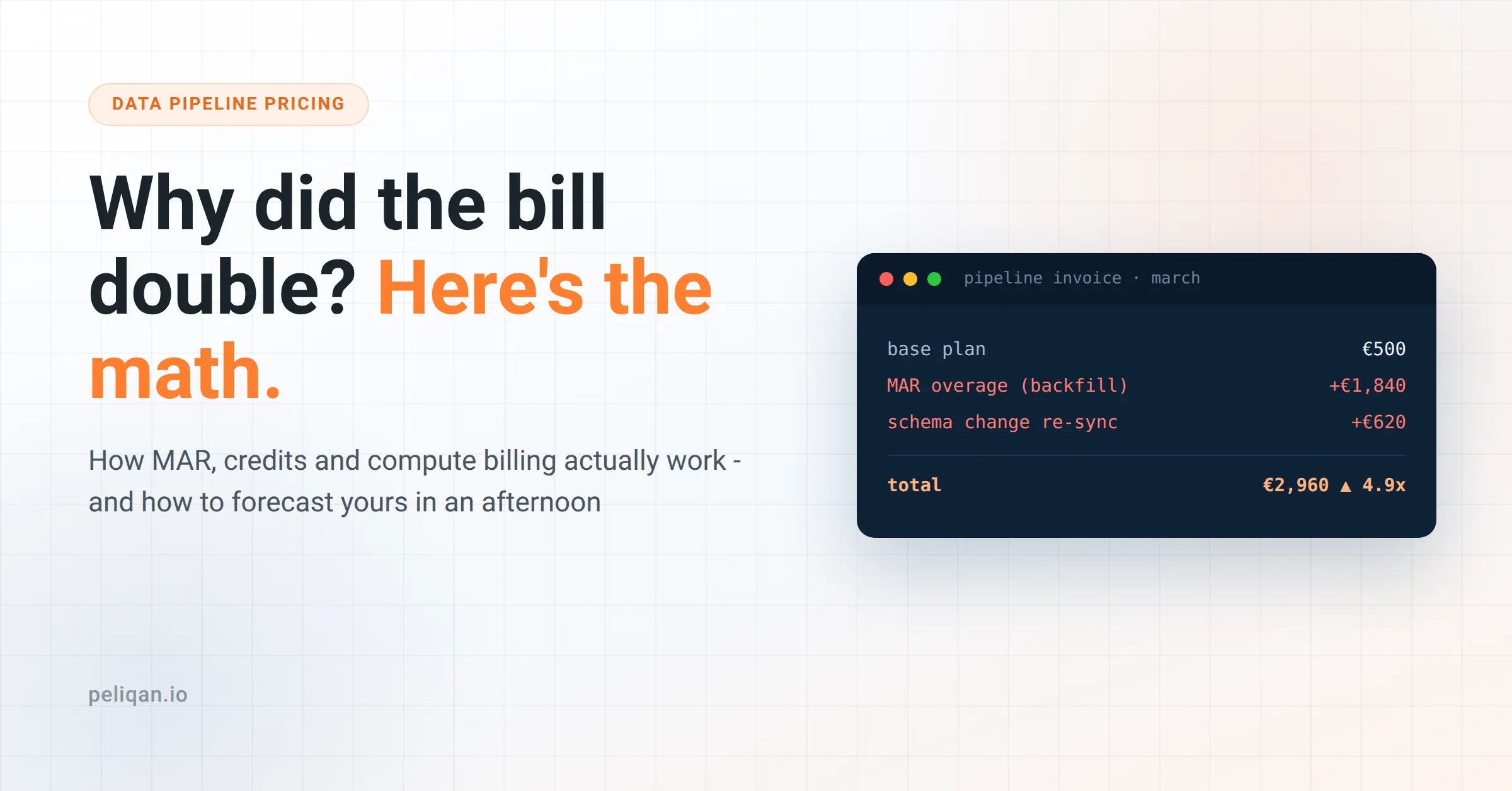





Data pipeline pricing comes in four flavors – active rows, event volume, credits and compute – and each one has a specific way of surprising you. This post explains how each model actually charges, why bills spike after backfills and schema changes, and how to forecast your own bill before you sign anything.
Almost every pipeline bill-shock story starts the same way. The tool worked, the team was happy, and then one invoice came in at three or four times the usual number.
Nobody changed the contract. Nobody added a warehouse. Someone added one connector, or re-synced one table, and the meter did the rest.
The frustrating part is that the spike was predictable – if you knew what the meter actually counts. Most teams don’t, because pricing pages explain the price per unit and stay quiet about what makes the units multiply.
So that is this post: what each data pipeline pricing model counts, the five mechanics that make bills jump, and a forecasting method you can run before choosing a tool. No villain story – usage pricing has honest uses too, and we’ll get to them.
The four data pipeline pricing models
Nearly every tool on the market charges one of four ways. The differences look small on a pricing page and enormous on an invoice.
There is a fifth model – a fixed monthly plan based on connections or users – which we’ll come back to, because it trades a different thing: you pay for headroom instead of usage.
One more thing the table hides: most stacks pay two of these meters at once. A row-based pipeline tool loading into a compute-billed data warehouse means your ingestion and your transformations each have their own way of spiking.
Snowflake’s own docs are refreshingly clear on the compute side: each warehouse size doubles the credits per hour, and you pay while it runs, working or not.
The five mechanics that make bills spike
These are the multipliers – the reason data pipeline pricing looks fine in month one and painful in month four. None of them are hidden, exactly. They are just never on the pricing page.
1. Backfills count as activity
Your first sync loads all historical data, and on row-based meters that history counts as active rows. Month one on a new connector is routinely the most expensive month it will ever have – which makes your trial-period bill a terrible predictor of steady state, in both directions.
2. Schema changes trigger re-syncs
A column added in your CRM, a type change in your ERP – many tools respond by re-syncing the whole table. Every row becomes active again. One innocent field added by an admin can replay your largest table through the meter.
3. High-churn tables dominate everything
The meter doesn’t care that a row is boring. Order statuses, stock levels, session records – rows that update constantly get counted constantly. In most companies, two or three churn-heavy tables produce the majority of the bill while the other hundred tables cost almost nothing.
4. Sync frequency multiplies volume meters
On meters that count records loaded rather than distinct rows, moving a table from daily to every 15 minutes can multiply its cost by up to 96. Freshness has a price; the question is whether anyone priced it before flipping the toggle.
5. Credits hide the exchange rate
Credit models – common among unified DataOps platforms – convert rows, gigabytes and operations into one abstract unit at a rate that varies by task. The unit price looks clean; the conversion is where forecasting dies. If you cannot state what one credit buys for your specific workload, you cannot forecast the bill – and that is not your failure, it is the model’s design.
How to forecast a data pipeline bill before you buy
You can get within useful range of your real data pipeline pricing in an afternoon. Five steps:
- Count your active rows at the source. Query each source table for rows created plus rows updated in the last full month. Most databases and SaaS admin views can answer this. This number, summed, is your steady-state MAR.
- Find your churn monsters. Rank tables by that number. The top three usually dominate – decide per table whether you need every update or a daily snapshot. Selective table syncing is the cheapest optimization that exists.
- Model month one separately. Total historical row counts = your backfill. Ask every vendor directly whether backfills and re-syncs count toward the meter, and get it in writing.
- Price your freshness. Decide sync frequency per table before the trial, not after. A 15-minute sync on one hot table plus daily on everything else costs a fraction of 15 minutes on all of it.
- Ask the five contract questions. What counts as active? Do backfills count? What happens on schema change? Do deleted rows count? Where are the volume-discount cliffs? A vendor who answers slowly is answering.
If your forecast still has a variance above roughly 30% after this exercise, that is information too: your workload is unpredictable enough that a usage meter will keep surprising you.
Usage pricing isn’t evil – unforecastable pricing is
Fairness matters here. Usage-based data pipeline pricing is genuinely the right model in some situations: tiny data volumes, spiky seasonal workloads, or experiments you may switch off next quarter. Paying per row for 50,000 rows a month beats any flat plan.
The problem is narrower than “usage bad”. It is that most usage meters are driven by events you do not control – a backfill, a schema change upstream, an admin adding a field – so the bill varies with things nobody budgeted. A meter you cannot forecast is not a price, it is a risk.
Fixed pricing has its own honest trade-off: you pay for headroom you may not use, and if your volumes are tiny, you are overpaying. The right question is not which model is cheaper but which failure mode you prefer – paying for unused headroom, or explaining a surprise invoice to finance. For most mid-market teams running steady data automation, headroom is the cheaper failure.
How we price Peliqan
Peliqan uses the fifth model: fixed monthly plans based on connections, where each database, warehouse or SaaS application counts as one connection – the full breakdown is on the pricing page.
Rows, syncs and backfills are not metered. There are no over-usage charges: if usage stays substantially above your package, we reach out to discuss an upgrade – the bill does not change by itself. Sync frequency is a setting, not a cost decision.
Transformations run in the built-in warehouse, so there is no second compute meter for SQL and Python transformations.
And for databases and warehouses, the federated query engine can query data live without storing a copy at all – the cheapest row is the one you never sync.
Stated honestly: if you sync 50,000 rows a month from two sources, a usage-metered tool will likely cost you less than any fixed plan, ours included. Fixed pricing earns its premium when volumes are real and finance wants a number that holds – which is most of the teams we work with, from 300+ connectors into one warehouse.
The bill is a design choice
Bill shock feels like bad luck, but data pipeline pricing is architecture. The meter you sign up for determines which ordinary events – a backfill, a new field, a hot table – become invoice events.
Run the afternoon forecast before your next renewal or trial. Whatever tool you land on, you’ll negotiate better knowing your own active rows than the vendor knowing them for you.
And if you want to see what your stack costs on a flat plan, book a demo – bring your source list, and we’ll map it to connections in the call. That number won’t change when someone adds a column.