Slow ETL pipelines don’t just delay dashboards – they stall every downstream decision that depends on fresh data. This guide covers the exact extraction, transformation, and loading techniques that cut pipeline run times by 50-75%, with code examples and architecture patterns you can apply today.

Data teams spend 44% of their time on data preparation and integration, according to Anaconda’s State of Data Science report. When ETL processes run inefficiently, that percentage climbs higher, creating bottlenecks that delay reporting cycles and frustrate stakeholders waiting on stale data.

The root cause is rarely a single failure point. It’s a combination of full-table extractions where incremental loads would suffice, row-by-row transformations that ignore vectorized operations, and static resource allocation that either wastes compute or starves critical jobs. Each of these problems compounds as data pipelines scale.

This guide breaks down ETL process optimization into its component parts – extraction, transformation, loading, orchestration, and monitoring – with specific techniques, SQL examples, and architecture decisions that separate fast pipelines from slow ones.

What ETL process optimization actually means

ETL process optimization is the systematic improvement of data extraction, transformation, and loading workflows to reduce latency, lower compute costs, and improve data quality at every stage. It covers three domains:

Technical tuning – parallelization, query rewriting, partitioning, caching, and index management within the pipeline code itself.

Architectural decisions – choosing between ETL and ELT patterns, selecting cloud-native vs. self-managed infrastructure, and designing staging layers that isolate failures.

Operational practices – monitoring, alerting, scheduling strategies, and continuous performance benchmarking against defined SLAs.

The goal is not abstract. It is to move the right data, at the right time, at the lowest cost, without sacrificing accuracy.

Baseline metrics: measure before you optimize

You cannot improve what you do not measure. Before changing anything, establish baselines for the following metrics and log them per pipeline run.

Log these metrics into a time-series store (Prometheus, CloudWatch, or even a dedicated table in your warehouse) so you can compare before and after any optimization change.

Optimizing extraction: pull only what changed

Extraction is the first bottleneck in most pipelines. The single highest-impact change you can make is switching from full-table extractions to incremental loading – processing only new or modified records since the last run.

Timestamp-based incremental extraction

If your source tables have a reliable updated_at column, filter extractions using a high-water mark – the timestamp of the last successful run:

SELECT *
FROM orders
WHERE updated_at > '2026-04-15 08:00:00'  -- last successful watermark
ORDER BY updated_at ASC;

Store the watermark value after each successful run. If the run fails, the watermark does not advance, so the next run reprocesses the same window – giving you automatic retry semantics.

Change data capture (CDC)

Timestamp-based extraction misses one critical event: deletes. If a record is removed from the source, a WHERE updated_at > X query will never surface it. CDC solves this by reading the database transaction log directly, capturing inserts, updates, and deletes as a continuous stream.

Log-based CDC (tools like Debezium reading MySQL binlog or PostgreSQL WAL) adds minimal load to the source system because it reads logs that the database already writes. This makes it the preferred approach for high-volume, low-latency requirements.

Extract only required columns

A common mistake is running SELECT * when only 12 of 80 columns are needed downstream. Explicitly listing columns in your extraction query reduces network transfer, memory consumption, and transformation processing time. On wide tables with LOB (large object) columns, this alone can cut extraction time by 40-60%.

Optimizing transformation: do less work, do it smarter

Transformation is where most compute resources are consumed. The optimization principles here are straightforward: process data in bulk, push work to the engine best suited for it, and eliminate redundant computation.

Replace row-by-row processing with set-based operations

Row-by-row processing (cursors in SQL, iterating with Python for loops over DataFrames) is the single most common performance killer in data transformation logic. Set-based SQL operations and vectorized library functions (pandas, Polars, DuckDB) process entire columns or tables at once, leveraging CPU caching and SIMD instructions.

-- Slow: cursor-based row update
DECLARE cur CURSOR FOR SELECT id, revenue FROM staging.orders;
-- ... row-by-row FETCH and UPDATE

-- Fast: single set-based UPDATE
UPDATE warehouse.fact_orders f
SET revenue_eur = s.revenue * fx.rate,
    is_valid    = CASE WHEN s.revenue > 0 THEN TRUE ELSE FALSE END
FROM staging.orders s
JOIN ref.exchange_rates fx ON s.currency = fx.currency_code
WHERE f.order_id = s.order_id
  AND s.updated_at > '2026-04-15 08:00:00';

Push transformations to the warehouse (ELT pattern)

Modern cloud data warehouses (Snowflake, BigQuery, Redshift, Postgres with columnar extensions) have massive compute capacity. Instead of extracting data, transforming it in a separate application, and then loading the result, the ELT pattern loads raw data first and runs transformations as SQL inside the warehouse.

This eliminates data movement between systems and leverages the warehouse’s MPP (massively parallel processing) architecture. For complex joins and aggregations, ELT typically delivers 2-5x performance improvements over traditional ETL because the warehouse can optimize query plans, use columnar storage, and parallelize across nodes automatically.

Cache expensive lookups

If your transformation joins against slowly-changing reference tables (country codes, product categories, exchange rates), cache these in memory rather than querying them for every batch. In Python pipelines, load reference data once into a dictionary. In SQL-based flows, materialize reference tables as indexed views or temporary tables at the start of each run.

Filter early, transform late

Apply WHERE clauses, column pruning, and null filtering as early in the pipeline as possible. Every row and column you eliminate before transformation reduces compute for every subsequent step. This is sometimes called “predicate pushdown” – pushing filter conditions down to the extraction query rather than filtering after loading everything into a staging area.

Optimizing loading: bulk, partition, index

Loading transformed data into the target system introduces its own set of bottlenecks: write contention, index maintenance overhead, and transaction log pressure.

Use bulk loading operations

Standard INSERT statements process one row per transaction. Bulk loading commands bypass this overhead:

-- PostgreSQL: COPY is 5-10x faster than row-by-row INSERT
COPY warehouse.fact_orders (order_id, customer_id, revenue_eur, order_date)
FROM '/tmp/transformed_orders.csv'
WITH (FORMAT csv, HEADER true, DELIMITER ',');

-- Snowflake: COPY INTO with staging
COPY INTO warehouse.fact_orders
FROM @my_stage/transformed_orders.parquet
FILE_FORMAT = (TYPE = 'PARQUET');

Parquet and Avro file formats compress data and preserve schema, reducing both transfer time and parsing overhead compared to CSV.

Partition target tables

Partitioning splits a large table into smaller physical segments based on a column value (typically date). This improves both write performance (the database only locks the relevant partition) and read performance (queries that filter on the partition key scan less data).

For a fact table partitioned by order_date, loading today’s data only touches today’s partition, leaving historical partitions untouched. This eliminates contention between ETL writes and analyst queries running against older data.

Manage indexes around loads

Indexes accelerate reads but slow down writes because the database must update every index on every insert. For large batch loads, a common pattern is to drop non-critical indexes before loading, then rebuild them after. On a 10-million-row load, this can reduce load time by 30-50%.

Parallel processing and partitioning

Parallelization is the single most scalable optimization technique. Instead of processing a 100M-row table sequentially, partition it into 10 segments of 10M rows each and process them concurrently across multiple workers.

Partition strategies

Range partitioning splits data by value ranges (date ranges, numeric ID ranges). Best for time-series data where recent partitions are written frequently and old partitions are read-only.

Hash partitioning distributes rows evenly across N partitions using a hash function on a key column. Best for achieving uniform parallelism when data distribution is skewed.

List partitioning assigns rows to partitions based on discrete values (region, country, business unit). Best when downstream consumers query by those dimensions.

Achieving linear scalability

With independent partitions, parallel ETL achieves near-linear scalability up to the point where I/O, network, or shared resources become the bottleneck. In practice, teams report 60-80% linear scaling – meaning 8 parallel workers complete the job in roughly 1.5x the time of a single worker instead of the theoretical 1x, due to coordination overhead.

The key constraint: tasks must be independent. If partition B depends on the output of partition A (for example, running totals across date ranges), you cannot parallelize them. Design transformations to be partition-independent wherever possible.

Staging areas and failure isolation

A staging area is a temporary holding zone between extraction and final loading. It serves two purposes: it isolates failures so a bad batch does not corrupt the production warehouse, and it provides a checkpoint for restart and recovery.

The three-layer pattern

Raw/landing layer: Extracted data lands here in its original format. No transformations. If extraction succeeds but transformation fails, you do not need to re-extract – just replay from this layer.

Staging/transform layer: Cleaned, validated, and transformed data lives here temporarily. Data quality checks run against this layer before anything is promoted to production.

Production/warehouse layer: Only data that passes all validation checks is loaded here. This is what analysts and BI tools query.

This pattern adds one extra write step but dramatically improves recoverability. If a transformation bug corrupts data in the staging layer, the raw layer is intact. If a load fails midway, the staging layer still holds the complete transformed batch for retry.

Error handling and recovery patterns

Production ETL pipelines fail. Sources go offline, schemas drift, API rate limits trigger, and data quality checks catch unexpected nulls. The difference between a resilient pipeline and a fragile one is how it handles these failures.

Pipeline orchestration

Orchestration is how you schedule, sequence, and manage dependencies between pipeline tasks. Moving beyond cron jobs to a proper orchestrator eliminates blind spots and enables event-driven execution.

DAG-based orchestration

Tools like Apache Airflow, Dagster, and Prefect model pipelines as directed acyclic graphs (DAGs) where each node is a task and edges represent dependencies. A DAG ensures that the transformation step does not start until extraction succeeds, and loading does not start until transformation completes and validation passes.

DAG-based orchestrators provide automatic retry on failure, dependency tracking, SLA monitoring, and historical run logs – all critical for operating pipelines at scale.

Scheduling strategies that reduce contention

Data quality checks inside the pipeline

Data quality is not a separate concern from performance optimization – it is part of it. Every invalid record that enters the pipeline consumes compute during transformation and storage space in the warehouse, only to produce incorrect downstream results that someone must debug and reprocess. Catching bad data early is both a quality and a performance optimization.

Where to place validation checks

Post-extraction: Validate schema conformity (expected columns, data types), check for nulls in required fields, and reject records that fail basic integrity rules. Route failures to a dead letter table.

Post-transformation: Run business rule validation – referential integrity checks, range checks (is revenue negative?), uniqueness constraints, and row count reconciliation between source and staging.

Post-loading: Compare record counts between staging and production. Run data quality monitoring queries to detect anomalies in freshly loaded data (sudden volume drops, unexpected nulls in previously populated fields).

Automated schema drift handling

Source systems change. APIs add fields, databases rename columns, and upstream teams alter data types. Without automated detection, these changes silently break pipelines or introduce nulls. Implement schema comparison at extraction time: compare the incoming schema against a stored baseline, auto-adapt for additive changes (new columns), and halt with an alert for breaking changes (dropped or renamed columns, type changes).

Monitoring and observability

A pipeline without monitoring is a pipeline waiting to fail silently. Observability covers three pillars: metrics (quantitative measurements), logs (event records), and traces (request-level flow tracking through pipeline stages).

Feed these metrics into dashboards (Grafana, CloudWatch, or your warehouse’s built-in monitoring) and set tiered alerts: warnings for degradation trends, critical alerts for SLA breaches or job failures.

SQL query optimization techniques

Inside the pipeline, poorly written SQL is a silent performance killer. These techniques apply whether you’re running transformations in a staging database or using the ELT pattern inside a cloud data warehouse.

Use explicit JOINs with indexed keys. Joining on non-indexed columns triggers full table scans. Ensure foreign key columns used in joins have indexes on both sides.

Replace correlated subqueries with JOINs or CTEs. A correlated subquery executes once per row in the outer query. Rewriting it as a JOIN or CTE allows the query planner to execute it once and hash-join the results.

Avoid SELECT DISTINCT as a fix for duplicates. DISTINCT forces a sort operation on the entire result set. If you’re getting duplicates, the root cause is usually a missing join condition or a bad extraction filter. Fix the source of duplicates rather than sorting them away.

Leverage warehouse-specific features. Snowflake’s automatic clustering, BigQuery’s partitioned tables, Redshift’s sort keys and distribution keys – these features can 10x query performance when configured correctly for your access patterns.

Use EXPLAIN/ANALYZE. Run your transformation queries through the query planner before deploying. Look for sequential scans on large tables (add indexes), nested loop joins on big datasets (restructure to hash joins), and excessive temporary disk spills (increase work memory or break the query into stages).

ELT vs. ETL: choosing the right architecture

The choice between ETL and ELT is an architectural decision that affects every optimization technique you can apply downstream.

Most modern teams use ELT as the default and apply ETL-style pre-processing only where compliance requirements demand it (masking PII before it enters the warehouse) or where source data requires non-SQL transformations (parsing XML, image processing, ML feature engineering).

Resource management and cost optimization

Over-provisioning wastes money. Under-provisioning causes failures and SLA breaches. The goal is right-sizing: allocating resources dynamically based on workload patterns.

Auto-scaling compute. Cloud warehouses like Snowflake offer auto-suspend (shut down compute after idle periods) and auto-resume (spin up on query arrival). For ETL workloads that run on a schedule, configure dedicated compute clusters that scale up during pipeline runs and scale to zero between them.

Separate ETL and analytics compute. Running ETL loads on the same cluster as analyst queries creates contention. Use separate warehouse clusters or materialization strategies – one sized for write-heavy ETL workloads, another sized for read-heavy analytics.

Compress data in transit and at rest. Parquet and ORC file formats compress data by 60-80% compared to CSV while preserving schema information. This reduces storage costs, network transfer time, and I/O during loading.

AI and automation in ETL optimization

Manual ETL optimization requires deep expertise and significant time investment. Modern platforms increasingly incorporate AI to automate repetitive optimization tasks:

Automated query plan analysis – AI reviews execution plans and recommends index changes, join reordering, or query rewrites.

Intelligent schema mapping – ML models suggest column mappings between source and target schemas, reducing manual mapping effort for new connectors.

Anomaly detection – Statistical models trained on historical pipeline metrics flag unusual execution times, row count drops, or resource spikes before they become incidents.

Natural language to SQL – For teams without dedicated data engineers, AI copilots convert business questions into optimized SQL queries, removing the bottleneck of hand-coding every transformation.

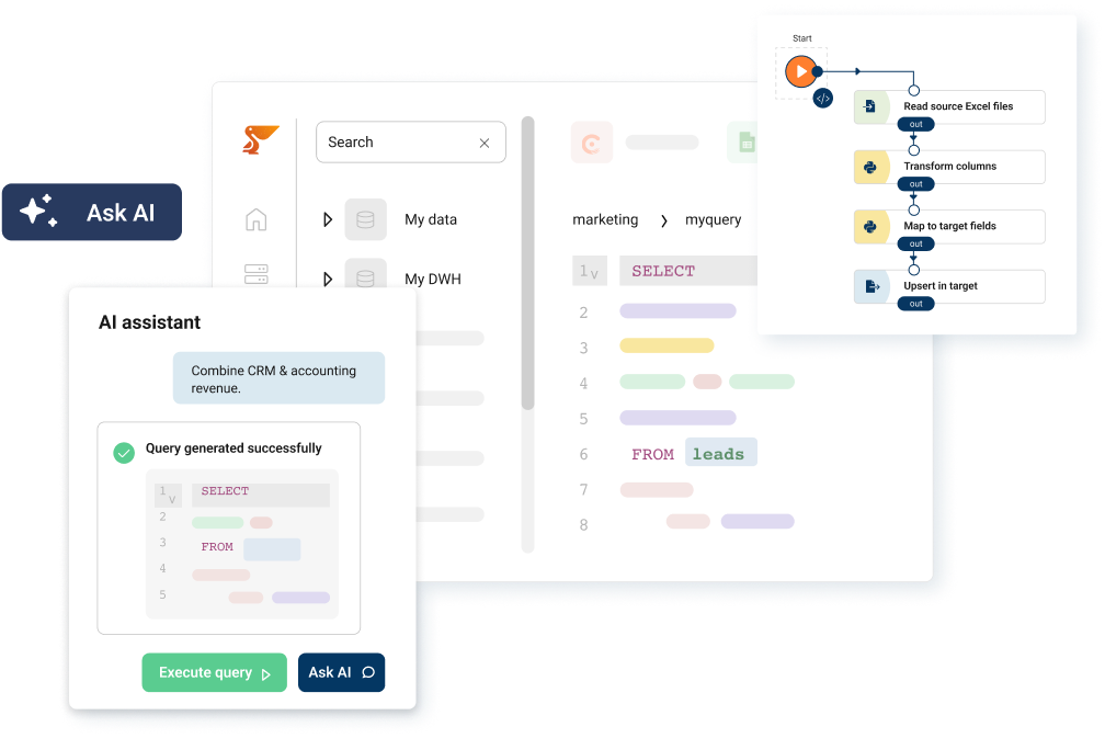
For organizations without dedicated data engineering teams, platforms like Peliqan provide AI-assisted data operations that convert natural language into optimized SQL and Python, apply automated data quality rules, and handle schema mapping across 250+ connectors – eliminating the need for deep pipeline engineering expertise while maintaining performance standards.

ETL optimization tools comparison

Choosing the right platform determines which optimization techniques are available out of the box vs. which require custom engineering. Here is how the leading ETL tools compare on optimization-specific capabilities:

Peliqan combines extraction, transformation, reverse ETL, and a built-in warehouse in a single platform – which eliminates the integration overhead and data movement between separate tools that often becomes its own optimization problem.

Performance benchmarks: what optimization delivers

The following benchmarks are composites from published case studies and industry reports. Your results will vary based on data volumes, source systems, and infrastructure, but they illustrate the magnitude of improvement each technique delivers.

Combined, these techniques routinely take pipelines from 4-6 hour run times down to under 1 hour. The OdooExperts case above is one example; teams that implement incremental loading and parallel processing together often see the most dramatic improvements because they address both volume and concurrency simultaneously.

Continuous optimization framework

ETL optimization is not a one-time project. Data volumes grow, source systems change, and business requirements evolve. Build a feedback loop:

Monthly metric review. Compare current pipeline latency, throughput, error rate, and cost against baselines. Identify any degradation trends before they become SLA breaches.

Quarterly architecture review. Evaluate whether current extraction strategies, transformation patterns, and data transformation approaches still match the workload. A table that was small enough for full refresh six months ago may now need incremental loading.

Test at 10x. Periodically run pipelines against a dataset 10x the current volume to identify bottlenecks before they hit production. This is where pipeline architecture decisions like partitioning and parallel processing prove their value.

Document every change. Keep a changelog of optimization changes with before/after metrics. This builds institutional knowledge and prevents teams from regressing to old patterns.

Conclusion

ETL process optimization is a combination of the right extraction strategy (incremental loading, CDC, column pruning), efficient transformation patterns (set-based SQL, ELT pushdown, caching), smart loading techniques (bulk operations, partitioning, index management), and operational discipline (monitoring, error handling, continuous review).

Start with the highest-impact change for your specific pipeline: if you’re running full-table extractions, switch to incremental loading. If transformations are slow, check for row-by-row processing and replace it with set-based operations. If loading is the bottleneck, implement bulk COPY and table partitioning.

For teams that want these optimizations built in from day one, Peliqan combines 250+ connectors, a built-in warehouse, SQL + Python transformations, reverse ETL, and AI-assisted optimization in a single platform – starting at ~$199/month with fixed pricing that does not scale with data volume.