Have you ever wished you could look back in time and see exactly how your data looked on a specific year, month, or even date? Modern businesses often need to analyze their data as it existed at a particular moment. For example, you might want to know which customers were active last January or what a project’s status was six months ago.

This kind of “time travel” analysis is not natively available in Power BI. However, it can be achieved with the right logic and design. In this article, we will explore how to simulate historical snapshots using the Slowly Changing Dimensions (SCD) Type 2 concept and two practical workarounds inside Power BI.

By the end, you’ll understand how to create “as-of” reporting that feels like a time machine within Power BI.

What is SCD Type 2 and Why It Matters

Data doesn’t stay the same forever. Customers change their address, employees move to new departments, and projects shift from “In Progress” to “Completed.” When this happens, we often need to know not just the latest value, but also what it was before and when the change took place.

This is where Slowly Changing Dimensions (SCD) come in. It’s a data warehousing technique used to track how dimension data evolves over time.

There are several types of SCDs, but Type 2 is the one that preserves a complete history of every version of a record. Instead of overwriting old values, it creates a new record whenever a change occurs and defines the period during which that version was valid.

Let’s look at a simple example. Imagine a table that stores customer information. On January 1st, ACME was recorded as “ACME Ltd.” A few days later, on January 15th, the name was updated to “ACME Inc.” Instead of losing the old record, both versions are stored like this:

Id   Name       City   Timestamp
1    ACME Ltd   NY     2024-01-01
1    ACME Inc   NY     2024-01-15

Now, if you want to see how your customer list looked on January 10th, you’ll see ACME Ltd. But if you pick February 1st, you’ll get ACME Inc. This is the foundation of the time-travel concept.

There are two main ways to bring this time-travel experience into Power BI. One uses Power Query, and the other uses DAX. They work a little differently but achieve the same goal. They let you see the data as it was on any given date.

Understanding the Challenge in Power BI

Most history tables store multiple versions of the same record, so the key challenge is figuring out which version was valid on that particular selected date. Power BI doesn’t natively let you say, “show me how the data looked on 2024-03-01.”

Many organizations maintain history tables that capture changes over time. A table like Employee_History or Customer_History might store multiple rows per entity, each representing its state at a different timestamp. The challenge is to let users pick a specific date and view the data exactly as it existed then, without creating a massive or unoptimized dataset.

Once we understand the problem, the next question is how to implement it efficiently.

When working in Import mode, bringing in multiple snapshots can quickly make the dataset huge and slow to refresh. On the other hand, in Direct Query mode, Power BI slicers cannot directly pass parameters into SQL queries, which makes dynamic date filtering difficult to achieve.

That’s why we need a smart design to make our as-of date logic work efficiently and interactively.

Two Ways to Build “Time Travel” in Power BI

There are two practical approaches to achieve a time-travel snapshot in Power BI with SCD Type 2 data.

1. M Query

This method uses Power Query (M) transformations along with a cutoff date parameter to pre-calculate the latest record for each ID as of a given date.
It’s ideal for creating static or scheduled snapshots, where you only need to refresh the report periodically.

Since the filtering and grouping occur before data is loaded into Power BI, this approach is usually faster and cleaner, especially when working with large datasets.

2. DAX

This approach uses a calendar table, a date slicer, and DAX measures to dynamically determine which records were valid as of the chosen date.
It’s perfect for interactive analysis, allowing users to move a date slider and instantly see how data looked on that day.

However, it requires more complex DAX logic and can impact performance if your dataset contains millions of history rows.

Creating a Sample Table with History Data

Before we dive into M Query or DAX logic, let’s first create a dummy SCD Type 2 table so you can experiment safely inside Power BI.

This dataset will simulate a real-world scenario where customer details change over time for example, when a customer updates its name or moves to a different city.

How to Create the Customer_History Table

1. Open Power BI Desktop
2. Go to Home → Transform Data
3. In Power Query, choose Home → New Source → Blank Query
4. Rename Blank Query as Customer_History
5. Open Advanced Editor and paste the following M code:

let
    Source = Table.FromRows({
        {1, "ACME Ltd", "NY", #date(2024, 1, 1), "1_2024-01-01"},
        {1, "ACME Inc", "NY", #date(2024, 1, 15), "1_2024-01-15"},
        {2, "Pepsi", "WA", #date(2024, 1, 1), "2_2024-01-01"},
        {2, "Pepsi Intl", "WA", #date(2024, 6, 1), "2_2024-06-01"},
        {3, "Cola", "BR", #date(2024, 1, 1), "3_2024-01-01"},
        {3, "Cola Corp", "BR", #date(2024, 8, 1), "3_2024-08-01"},
        {4, "Hooli", "CA", #date(2024, 1, 1), "4_2024-01-01"},
        {4, "Hooli Labs", "CA", #date(2024, 7, 1), "4_2024-07-01"},
        {5, "Initech", "OH", #date(2024, 1, 1), "5_2024-01-01"},
        {5, "Initech Ltd", "OH", #date(2024, 6, 15), "5_2024-06-15"},
        {6, "Umbrella", "IL", #date(2024, 1, 1), "6_2024-01-01"},
        {6, "Umbrella Inc", "IL", #date(2024, 9, 1), "6_2024-09-01"},
        {7, "Soylent", "TX", #date(2024, 1, 1), "7_2024-01-01"},
        {7, "Soylent Max", "TX", #date(2024, 5, 1), "7_2024-05-01"},
        {8, "Globex", "FL", #date(2024, 1, 1), "8_2024-01-01"},
        {8, "Globex Corp", "FL", #date(2024, 3, 1), "8_2024-03-01"},
        {9, "Stark", "NY", #date(2024, 1, 1), "9_2024-01-01"},
        {9, "Stark Ltd", "NY", #date(2024, 4, 1), "9_2024-04-01"},
        {10, "WayneTech", "NJ", #date(2024, 1, 1), "10_2024-01-01"},
        {10, "Wayne Global", "NJ", #date(2024, 7, 1), "10_2024-07-01"},
        
    },
    {"Id", "Name", "City", "Timestamp", "History id"}),
    #"Changed Type" = Table.TransformColumnTypes(Source,{{"Timestamp", type date}, {"Id", Int64.Type}})
in
    #"Changed Type"

Click Close Apply to load the table.

Your Customer_History table now contains multiple versions of each record with different timestamps.

Method 1: Building the “As-of-Date” Snapshot in Power Query

In SQL, we usually write snapshot logic like this:

SELECT DISTINCT ON (id) *
FROM customer_history
WHERE timestamp < '2024-12-25T00:00:00'
ORDER BY id, timestamp DESC;

You can perform the same logic in Power Query (M Query) using filtering, sorting, and grouping.

• Filtering rows where [Timestamp] <= CutoffDate
• Sorting by Id and Timestamp descending
• Grouping by Id and keeping only the first row per group

Let’s implement this step-by-step.

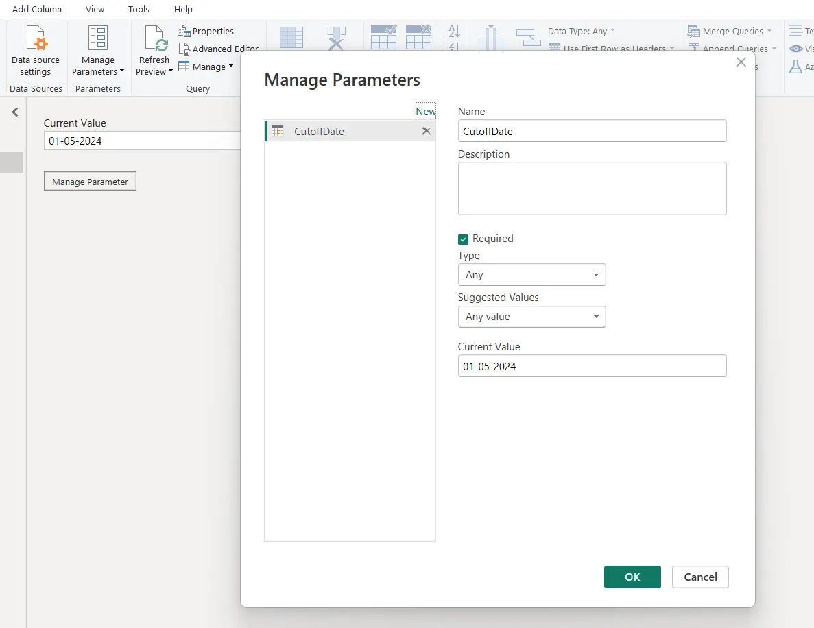
Step 1: Create a Cutoff Date parameter

Navigate to Manage Parameters → New Parameter and configure the following:

• Name: Cutoff Date
• Type: Date
• Current Value: e.g., 01-05-2024

This defines the “as-of” date for the snapshot.

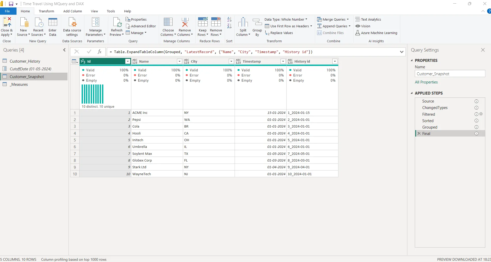
Step 2: Create the snapshot table in M Query

Power Query → New Source → Blank Query → Rename: Customer_Snapshot

Open Advanced Editor and paste:

let
// STEP 1: Reference the Customer_History table
Source = Customer_History,
// STEP 2: Convert types
ChangedTypes = Table.TransformColumnTypes(Source, {
    {"Id", Int64.Type},
    {"Name", type text},
    {"City", type text},
    {"Timestamp", type date},
    {"History id", type text}
}),

// STEP 3: Filter rows that are valid on or before the selected CutoffDate
Filtered = Table.SelectRows(ChangedTypes, each [Timestamp] <= CutoffDate),

// STEP 4: Sort by Id ascending and Timestamp descending
// History id is added as a tie breaker
Sorted = Table.Sort(
    Filtered,
    {
        {"Id", Order.Ascending},
        {"Timestamp", Order.Descending},
        {"History id", Order.Descending}
    }
),

// STEP 5: Group by Id and take the latest record for each Id
Grouped = Table.Group(
    Sorted,
    {"Id"},
    {{"LatestRecord", each Table.FirstN(_, 1), type table}}
),

// STEP 6: Expand the latest snapshot record
Final = Table.ExpandTableColumn(
    Grouped,
    "LatestRecord",
    {"Name", "City", "Timestamp", "History id"}
)

in
    Final

Click Close Apply

Now the Customer_Snapshot table contains 1 row per Id, valid as-of the selected date.

Verification Tip

To confirm your snapshot logic:

• Pick a few IDs and cross-check them in the original History table.
• For each ID, you should see only the record with the most recent Timestamp that’s ≤ CutoffDate.
• Change the parameter (for example, to 2024-09-01) and refresh your snapshot will automatically update.

In our example, the Cutoff Date was 01-05-2024, so in the Customer_Snapshot table we can now see the latest snapshot (version) of each record as of that date.

Now you have a Customer_Snapshot table that returns one record per ID, valid as of the selected date.
Change the parameter anytime to regenerate a new snapshot view.

Advantages:

• Produces a clean, static snapshot you can export or reuse.
• Keeps the logic transparent at the table level.

Limitations:

• Updates only when you refresh the model or change the parameter.
• Not interactive (can’t change from a slicer in the report).

Method 2: DAX Measures for Dynamic Filtering

Now let’s move to the second method using DAX to achieve an interactive time-travel experience directly in Power BI visuals.

Step 1: Verify the History Table

Use the same Customer_History table created earlier. This table serves as the historical data source for time-travel analysis.

Step 2: Create a Calendar Table

To allow time-based filtering, create a dedicated Calendar table that spans your entire date range:

Calendar =
CALENDAR(
MIN('Customer_History'[Timestamp]),
MAX('Customer_History'[Timestamp])
)

Step 3: Mark the Calendar as a Date Table

1. Go to Model View
2. Select the Calendar table
3. Choose Mark as Date Table
4. Select the [Date] column

This ensures DAX time intelligence functions like (SELECTEDVALUE or MAX) work accurately.

Step 4: Create the DAX Measure for Latest Records

Now, create a measure that dynamically identifies which version of each project was valid on the date selected in the slicer:

LatestAsOfCutoff = 
VAR CutoffDate = SELECTEDVALUE(Calendar[Date])  
    // Gets the date the user selected in the slicer

VAR LatestTimestamp = 
    CALCULATE(
        MAX('Customer_History'[Timestamp]),               
        FILTER(
            ALL('Customer_History'),                      
            'Customer_History'[Id] = MAX('Customer_History'[Id]) &&  
                // For the same ID as the current row
            'Customer_History'[Timestamp] <= CutoffDate     
                // Only include records on or before the selected date
        )
    )
    // Finds the latest timestamp for that ID up to the cutoff date

RETURN
    IF(
        MAX('Customer_History'[Timestamp]) = LatestTimestamp,
        1,   // This row is the latest as of the cutoff date
        0    // This row is an older version
    )

Above measure returns 1 for records that were active as of the selected cutoff date.

Step 5: Apply the Measure in Visuals

1. Add a date slicer using Calendar[Date]
2. Add a table or matrix visual showing company details from Customer_History
3. Drag the measure LatestAsOfCutoff into the Filters pane
4. Set the filter to “is 1”

Now, when you move the date slicer, all visuals instantly update to reflect the historical state of your customers as of that chosen date.

⚠️Do not create a relationship between the Calendar table and the Customer_History table when you are using the DAX method.

The table on the left side of your report should show the complete history, and the table on the right side should show the Customer_Snapshot based on the date selected in the slicer. This layout helps you compare how the snapshot changes when the user adjusts the slicer.

Why should you avoid the relationship

The DAX measure must read the entire history table without any filters so it can correctly identify the latest valid record for each Id on the selected date.

If you connect the Calendar table to the Customer_History table, then the slicer will filter the history table before the measure is evaluated. This removes the rows that the measure needs, which leads to incorrect snapshots or blank results.

Advantages:

• Fully interactive and it responds instantly to slicer changes.
• Perfect for analysis and visual storytelling.

Limitations:

• Works only at the visual level (doesn’t create a physical snapshot).
• You need a separate measure for each historical table (Projects, Customers, etc.).

Conclusion

Both methods for building time-travel reporting in Power BI come with their own trade-offs.

Power Query offers clean snapshots but lacks flexibility because results are fixed at refresh time.

DAX provides dynamic evaluation but demands careful use of measures across all visuals to avoid incorrect results.

Working with SCD Type 2 data is not always straightforward, and choosing the right approach depends on the level of flexibility and maintenance you want. In the next part, we will look at techniques that make point-in-time reporting easier to manage and more reliable across different scenarios.