Data vault modeling is a warehouse design pattern built for sources that change, schemas that drift, and audit trails that have to hold up under regulator scrutiny. It splits the warehouse into three primitives – hubs, links, and satellites – and uses hash keys to load them in parallel without sequential dependencies. This guide covers what data vault modeling actually is in 2026, how Data Vault 2.0 differs from the original spec, the SQL patterns that hold up in production on Snowflake, BigQuery, and Databricks, and where it fits next to Kimball, Inmon, and the wide-table approaches that have come back into fashion.

What is data vault modeling?

Data vault modeling is an enterprise warehouse design method introduced by Dan Linstedt in 2000, with the Data Vault 2.0 specification published in 2013. It separates business keys, relationships, and descriptive attributes into three table types so that source-system changes don’t ripple through the warehouse and historical accuracy is preserved by design.

The core idea: a warehouse should be able to absorb a new source, a renamed column, or a fresh business rule without rewriting existing tables. That’s the audit-friendly, schema-tolerant property regulators care about (NIS2, SOX, GDPR) and that data engineers care about when sources change quarterly.

Data vault sits next to other warehouse modeling approaches rather than replacing them. Most production setups use it as the foundational raw layer and then materialize Kimball-style facts and dimensions on top for analytics consumers.

The three building blocks

Hubs – business keys, immutable, deduplicated

A hub stores the unique business keys for a single business concept (Customer, Order, Product). Hubs are intentionally narrow: a hash key, the natural business key, a load timestamp, and the source system. No descriptive attributes, no relationships – those go in satellites and links respectively.

CREATE TABLE Hub_Customer (
    Customer_HK     CHAR(32)     NOT NULL,  -- MD5/SHA-256 hash of Customer_BK
    Customer_BK     VARCHAR(50)  NOT NULL,  -- natural business key
    Load_Date       TIMESTAMP    NOT NULL,
    Record_Source   VARCHAR(100) NOT NULL,
    CONSTRAINT PK_Hub_Customer PRIMARY KEY (Customer_HK)
);

Hub design rules that hold up in production: one business concept per hub, hash key derived deterministically from the business key (so the same customer in two systems gets the same hash), and at least one satellite attached to every hub. Empty hubs without satellites are a structural smell.

Links – many-to-many relationships between hubs

A link captures the relationship between two or more hubs. Verbs in the business language – Customer-places-Order, Order-contains-Product, Employee-manages-Department – all become links. Like hubs, links are sparse: hash keys for the parent hubs, a hash key for the link itself, load metadata, and that’s it.

CREATE TABLE Link_Order_Product (
    Link_OP_HK      CHAR(32)     NOT NULL,
    Order_HK        CHAR(32)     NOT NULL,
    Product_HK      CHAR(32)     NOT NULL,
    Load_Date       TIMESTAMP    NOT NULL,
    Record_Source   VARCHAR(100) NOT NULL,
    CONSTRAINT PK_Link_OP PRIMARY KEY (Link_OP_HK)
);

Variants worth knowing: same-as links connect two business keys that turn out to be the same entity (Customer 12345 in CRM = Customer C-9988 in billing); hierarchical links capture parent-child relationships within a single hub; non-historized links are used for events that don’t need historical tracking (each event is its own immutable row).

Satellites – descriptive attributes and history

Satellites carry the descriptive context for hubs and links: customer name, address, phone, product price, order status. They’re the only place where attribute history accumulates. When the source changes, a new satellite row is inserted with a fresh load timestamp – the old row stays.

CREATE TABLE Sat_Customer_Profile (
    Customer_HK     CHAR(32)     NOT NULL,
    Load_Date       TIMESTAMP    NOT NULL,
    Load_End_Date   TIMESTAMP,                        -- effective-end for current row
    Hash_Diff       CHAR(32)     NOT NULL,            -- attribute hash for change detection
    Customer_Name   VARCHAR(100),
    Email           VARCHAR(150),
    Phone           VARCHAR(50),
    Country         VARCHAR(50),
    Record_Source   VARCHAR(100) NOT NULL,
    CONSTRAINT PK_Sat_Customer_Profile PRIMARY KEY (Customer_HK, Load_Date)
);

Common practice is to split satellites by rate of change and by source: fast-changing fields (status, last login) get their own satellite; slow-changing fields (name, country) get another; a separate satellite per source system avoids cross-source attribute mixing.

Data Vault 2.0 – what changed

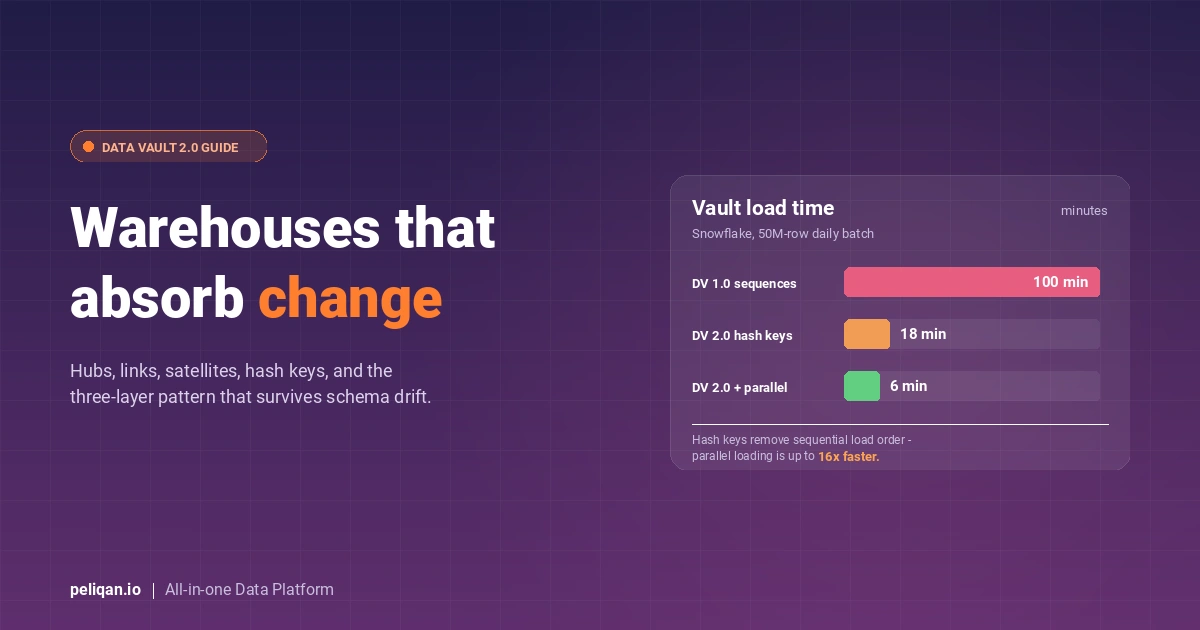
The original 2000 spec used database sequence numbers as primary keys, which forced sequential loading: load hubs first, then links, then satellites. Data Vault 2.0 replaced sequences with deterministic hash keys, which removed the sequential dependency entirely. Modern platforms – Snowflake, Databricks, BigQuery – can now load hubs, links, and satellites in parallel because the hash key for a record is computable from the source data without consulting the warehouse.

Hash keys are computed in the loading pipeline, not the warehouse. A typical pattern uses MD5 or SHA-256 of the trimmed, upper-cased business key concatenated with a separator. Two records from two systems with the same logical business key produce the same hash, which is what makes parallel loading and cross-system joins possible.

Raw vault vs business vault vs information marts

The biggest mistake in real-world data vault implementations is treating it as one flat layer. Data Vault 2.0 explicitly defines three:

Skipping the business vault tends to push business logic into individual marts, which is exactly the duplication that data vault was designed to prevent. Skipping information marts pushes complex hub-link-satellite joins onto BI tools, which kills query performance. The three-layer design exists because each layer absorbs a different kind of change.

Point-in-time tables and bridge tables

Querying a data vault directly requires joining hubs, links, and satellites with effective-dating logic – which gets expensive fast. Two helper structures fix this:

Point-in-time (PIT) tables precompute, for a given date, which satellite row was active. A PIT for Customer might have one row per customer per snapshot date, with foreign keys to the satellite versions current at that date. Queries that ask “what was the customer’s address on 2026-03-15” become a single PIT lookup instead of a windowed satellite scan.

Bridge tables precompute join paths between hubs through links. If a query frequently goes Customer-Order-Product, a bridge table flattens that traversal so the query is one join instead of three.

Both PIT and bridge tables are derived structures – they live in the business vault or information marts, get rebuilt on a schedule, and never get hand-edited. They’re optimization, not design.

Data vault vs Kimball vs Inmon – when to choose what

The strongest production patterns are hybrid: data vault as the raw and business vault layer for source-tolerance and audit, with Kimball-style information marts on top for query performance. The vault absorbs source change; the marts absorb consumer change.

Implementation – a worked e-commerce example

Step 1: identify business keys and create hubs

Walk the source systems and pull out the natural business keys for each concept that exists across them. For an e-commerce business: Customer (email or customer ID), Order (order ID), Product (SKU). One hub per concept, regardless of how many systems carry it.

CREATE TABLE Hub_Order (
    Order_HK        CHAR(32)     NOT NULL,
    Order_BK        VARCHAR(50)  NOT NULL,
    Load_Date       TIMESTAMP    NOT NULL,
    Record_Source   VARCHAR(100) NOT NULL,
    CONSTRAINT PK_Hub_Order PRIMARY KEY (Order_HK)
);

-- Insert pattern: only insert if Order_HK doesn't already exist
INSERT INTO Hub_Order (Order_HK, Order_BK, Load_Date, Record_Source)
SELECT
    MD5(UPPER(TRIM(Order_BK))) AS Order_HK,
    Order_BK,
    CURRENT_TIMESTAMP,
    'shopify'
FROM staging.shopify_orders s
WHERE NOT EXISTS (
    SELECT 1 FROM Hub_Order h
    WHERE h.Order_HK = MD5(UPPER(TRIM(s.Order_BK)))
);

Step 2: model relationships as links

For each business event, define the link. An order containing a product becomes Link_Order_Product; a customer placing an order becomes Link_Customer_Order. Links never carry descriptive context – that goes in satellites attached to the link.

Step 3: organize attributes into satellites by rate of change

Don’t put every column in one satellite. Split by rate of change and by source: a Sat_Product_Core for stable fields (name, brand, category), a Sat_Product_Pricing for volatile fields (price, discount), and source-specific satellites if the same product comes from two systems with different fields.

CREATE TABLE Sat_Product_Pricing (
    Product_HK      CHAR(32)     NOT NULL,
    Load_Date       TIMESTAMP    NOT NULL,
    Load_End_Date   TIMESTAMP,
    Hash_Diff       CHAR(32)     NOT NULL,
    Price           NUMERIC(10,2),
    Currency        CHAR(3),
    Discount_Pct    NUMERIC(5,2),
    Record_Source   VARCHAR(100) NOT NULL,
    CONSTRAINT PK_Sat_Product_Pricing PRIMARY KEY (Product_HK, Load_Date)
);

The full implementation walkthrough covers staging, hash key generation, and orchestration in more detail.

Loading patterns that work in production

Strong data lineage coverage is what makes this load pattern operationally tolerable. Every row carries its load timestamp and source system, so when a downstream report disagrees with a source-system query, you can trace exactly when and from where each value arrived.

Automation tools – what teams actually use

The automation tools all converge on the same idea: a data vault is repetitive enough that hub/link/satellite SQL should be generated from metadata, not handwritten. Teams that hand-roll often regret it by source #20.

Common challenges and concrete fixes

The AI era – data vault and MCP

AI agents are now legitimate consumers of warehouse data alongside dashboards. The properties that made data vault attractive for analytics – schema tolerance, source traceability, audit trails – are exactly the properties agents need to answer questions reliably.

The implementation pattern that’s emerging: keep the raw and business vault as-is, generate semantic-layer information marts that an MCP server exposes to agents, and let the agent ask “what was customer 12345’s order history” without ever touching hub-link-satellite joins. Lineage flows through the layers, so a question that an agent answers can be traced back to a specific source row with a load timestamp.

This is where metadata-driven semantic layers become load-bearing. The agent doesn’t need to know what a satellite is. It needs to know “customer email” maps to a column, that column has a definition, and the definition is current.

Real-world implementation

Most data vault projects fail not because the model is wrong, but because the operational footprint is heavy: connectors, staging, hash key generation, raw vault loaders, business vault transforms, PIT/bridge maintenance, and information mart materialization across 4-6 different tools.

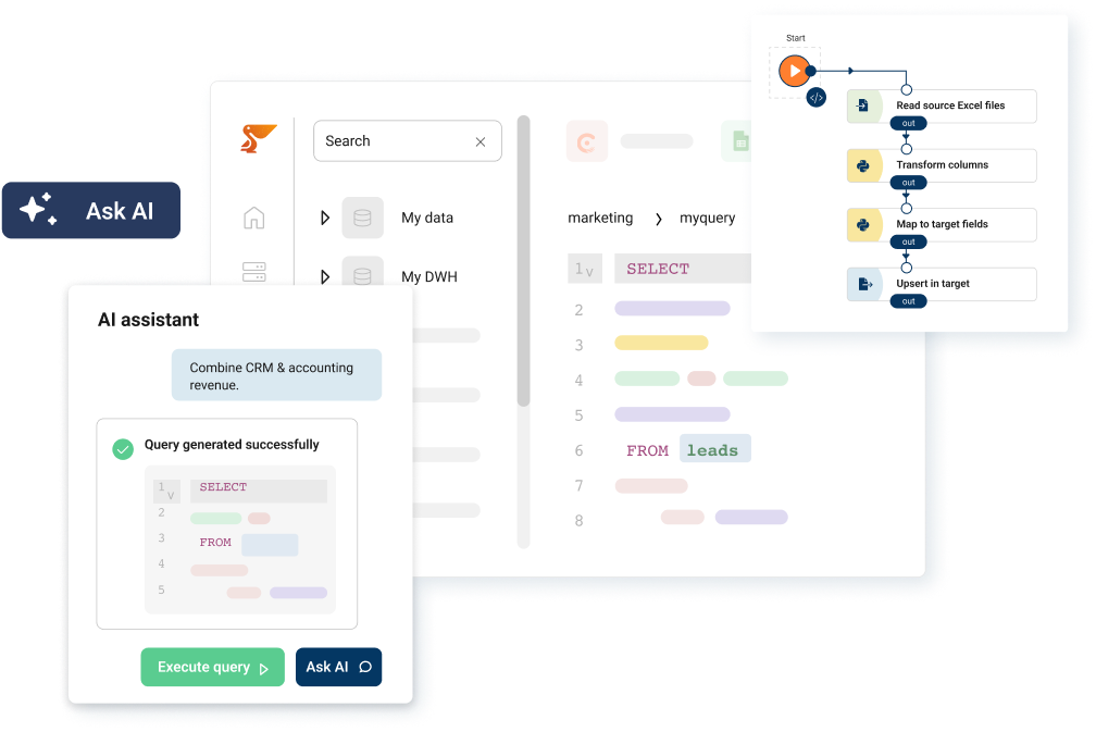
Peliqan consolidates that into one platform – 250+ connectors feeding a built-in Postgres/Trino warehouse, low-code SQL/Python transformations for raw and business vault layers, and materialized table support for information marts. Reverse-ETL and APIs come included for activating the marts back into operational tools.

The use cases that benefit most: regulated industries dealing with NIS2, GDPR, or SOC 2 compliance; multi-entity finance teams consolidating ERPs; SaaS platforms doing customer data resolution; investment firms tracking portfolio performance; and enterprise data warehousing efforts that combine data from multiple sources with frequent schema change.

When data vault is overkill

Don’t use data vault for: a single-source warehouse with stable schemas, a small analytics use case where time-to-first-dashboard matters more than long-term flexibility, or a team without the engineering bandwidth to maintain a three-layer architecture. The startup-tax of data vault is real, and it pays back over years – not weeks.

The decision usually comes down to source count, schema volatility, regulatory pressure, and warehouse lifespan. If three of those four are high, data vault earns its keep. If only one is, simpler patterns built directly on a data warehouse architecture usually win.

Monitoring and maintenance

A production data vault needs the same observability discipline as any other pipeline: row counts per layer, freshness per satellite, hash collision audits (rare but worth tracking), automation in data processing and load orchestration, and an alerting flow for missing or stale loads.

Beyond the basics: track the ratio of insert to update workload (should be 100% insert in raw vault), the hash diff hit rate (high hit rate means few real changes – useful for capacity planning), and the time between source-of-truth update and information mart materialization (your real-time reporting SLA depends on this).

Conclusion

Data vault modeling is a long-game choice. It pays back when source counts climb, schemas drift, audit requirements tighten, and the warehouse needs to outlast multiple generations of source systems and BI tools. Data Vault 2.0’s hash keys and three-layer architecture make it operationally viable on cloud warehouses in a way the original spec wasn’t.

The teams that succeed with it pick automation early, accept the operational cost of three layers, and resist the temptation to query the raw vault directly. The teams that struggle treat it as a star schema with extra steps, hand-roll the loaders, and skip the information mart layer.

It’s not the right choice for every warehouse. When it is the right choice, no other pattern absorbs change as gracefully or holds up to audit as cleanly. The model has been in production at scale for over two decades because the underlying problem it solves – decoupling business concepts from source-system schemas – hasn’t gone away. If anything, in an era of data integration across hundreds of SaaS apps, AI agents as warehouse consumers, and accelerating regulatory pressure, the case is stronger now than when Linstedt published the original spec. Reference implementations are widely covered in academic resources like data vault modeling literature for teams that want to dive deeper into the formal definitions.